PPP with RTKLIB and local correction
This is now my third attempt to get an exact position of my fixed mounted GNSS antenna at the roof of my house.
You can find the methods I used previously in my blogs here:
(1) PPP - Precise Point Positioning with averaging
(2) PPP with gpsrinex and CSRS-PPP and ECIT
As GNSS receiver I used again my u-blox ZED-F9P
to manage this device I use the gpsd package.
This time I used RTKlib to make the post-processing by myself. There are different versions available, I used this: github.com/rtklibexplorer/RTKLIB
The method is about this:
1) create an UBX file over several hours.
2) apply the correction with a RINEX file offered from an external service provider.
Within a shell script I prepared my ZED-F9P with the following settings:
check if baud-rate is high enough
ubxtool -g CFG-UART1-BAUDRATE | grep CFG-UART1-BAUDRATE
I use 921600 bd. This is the highest value I can use. 38400 would be the default.
now disable NMEA protocol and check the response
ubxtool -d NMEA | grep UBX-ACK-ACK:
ubxtool -z CFG-UART1OUTPROT-NMEA,0 | grep UBX-ACK-ACK:
ubxtool -g CFG-UART1OUTPROT-NMEA | grep CFG-UART1OUTPROT-NMEA | head -1
enable or disable different satellites
I disabled Michibiki, the japanese satellites as I can see them very rarely.
ubxtool -z CFG-SIGNAL-SBAS_L1CA_ENA,1 | grep UBX-ACK-ACK:
ubxtool -z CFG-SIGNAL-SBAS_ENA,1 | grep UBX-ACK-ACK:
ubxtool -z CFG-SIGNAL-QZSS_L1CA_ENA,0 | grep UBX-ACK-ACK:
ubxtool -z CFG-SIGNAL-QZSS_L1S_ENA,0 | grep UBX-ACK-ACK:
ubxtool -z CFG-SIGNAL-QZSS_L2C_ENA,0 | grep UBX-ACK-ACK:
ubxtool -z CFG-SIGNAL-QZSS_ENA,0 | grep UBX-ACK-ACK:
ubxtool -g CFG-SIGNAL | sed -n -e '/^UBX-CFG-VALGET:/,/^$/ p' | awk -v RS= 'NR==1'
enable raw data
ubxtool -e RAWX | grep UBX-ACK-ACK:
ubxtool | grep RAWX
to get satellite track data
ubxtool -e SFRBX | grep UBX-ACK-ACK:
ubxtool -z CFG-MSGOUT-UBX_RXM_SFRBX_UART1,1 | grep UBX-ACK-ACK:
SECS=50400
DAT=`date '+%Y%j%H%M00'`
FILE=`echo result$DAT`
gpspipe -x $SECS -R gpsdhost:gpsd:/dev/serial0 > $FILE.ubx
This gpspipe job will run 14 hours. ( = 50400 seconds )
Next is to generate $FILE.obs , $FILE.nav and $FILE.sbs To do this run convbin
convbin $FILE.ubx
Instead of convbin one can run the GUI rtkconv_qt & interactive.
If files $FILE.obs and $FILE.nav are available one can view some graphs with
rtkplot_qt -r $FILE.obs $FILE.nav &
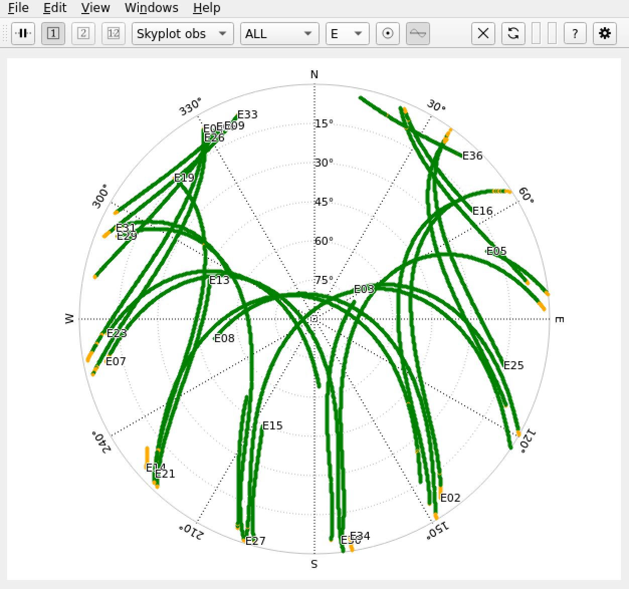
For example the skyplot for Galileo for the period of 14 hours.
Now comes the part of preparing the correction.
For this we need the RINEX (Receiver Independent Exchange Format) data from a reference station. I use the APOS-PP from BEV. BEV is the Federal Office of Metrology and Surveying ( Bundesamt für Eich- und Vermessungswesen ) in Austria and APOS-PP is a free service they offer. APOS-PP is the Austrian Position Service Post Processing. See APOS
The free available RINEX files are accessible short time after 00:00 UTC, so I fetched them next day. As there are about 60 reference stations one has to select a station which is near to the own position. In my case it’s WIEN00AUT. As each file has only 1 hour of data therefore multiple files are needed. The files have type .crx.gz. To get a .rnx run first gunzip and than CRX2RNX. CRX2RNX is also free available and should have at least version : ver.4.2.0. Older Versions are buggy. Finally all these files have to be combined to one file. This is done with gfzrnx which is also free available. Current available VERSION: gfzrnx-2.2.0 at GFZ.de
Now comes the real part of correction. There are 2 possibilities:
- a GUI
rtkpost_qt - a command line tool:
rnx2rtkp
As first step I run the GUI. The reason is that some settings can be saved in a configuration file which can be used with the command line tool as argument. I configured under “Setting1” position mode “Static” and selected Navigation Systems: GPS, Galileo, Glonass and BDS. In selector “Positions” I entered below “Base Station” the position in X/Y/Z-ECEF format ( Earth-Centered, Earth-Fixed ). The values can be found in the final .rnx file in line marked with APPROX POSITION XYZ. Don’t worry, it’s not approximately, it is exact. In case of WIEN00AUT it is 4085097.7110 1200224.1682 4733306.7362. It’s important to enter the exact values, otherwise the calculated result is wrong. Now press the “Save” button and give the configuration file a name, e.g. “myconfig.conf”. Back to the main window enter the necessary file names. It is the .obs file for Rover, the .rnx file for the basestation and also needed .nav and .sbs file. In the solutions sections you get a proposal for the final position file name. Press the “Execute” button. After a while - maybe a minute - you get the result. Press the “Plot” button. It will start rtkplot_qt with the .pos file. If “Ground Track” is selected we can see that the position goes around only few centimeter during the last hours. Better to see using the “Position” tab.
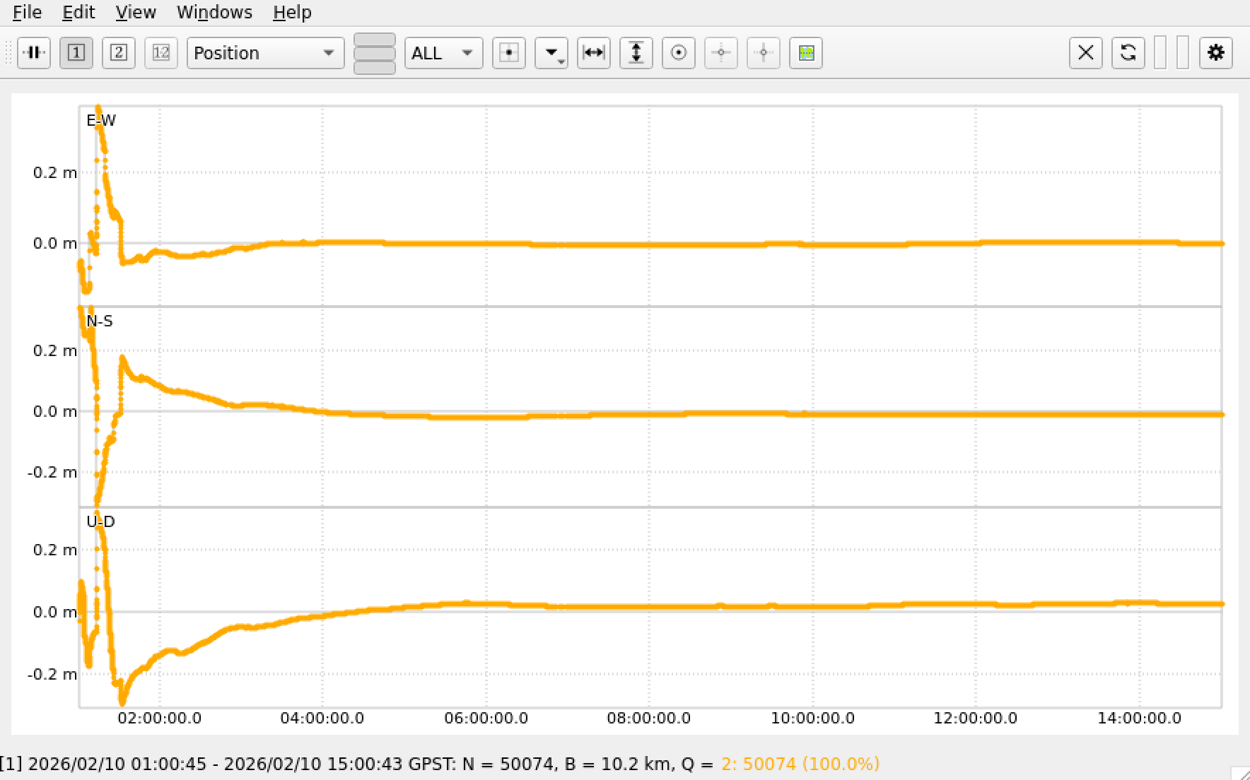
As we can see the curve swings in. As value I don’t use the last line of the result file, I use the average of the last 3 hours. Especially don’t use the first 2 lines for calculating the average.
Instead of using the GUI with rtkpost_qt it’s also possible to use the command line tool rnx2rtkp. As we have now a config file we can apply this as argument with option -k calling rnx2rtkp. A typical call looks like this:
rnx2rtkp -k myconfig.conf -o $FILE.pos $FILE.obs $FILE.rnx $FILE.nav $FILE.sbs
I run this scenario over several days. And this is the result
| date | longitude | latitude | altitude |
|---|---|---|---|
| result2026031081521.pos | 48.14928692997 | 16.28383533848 | 286.24190831482 |
| result2026035020026.pos | 48.14928677086 | 16.28383492415 | 286.22960926852 |
| result2026036020000.pos | 48.14928679808 | 16.28383546030 | 286.25004589815 |
| result2026037020000.pos | 48.14928691925 | 16.28383549683 | 286.25375274075 |
| result2026038020000.pos | 48.14928667076 | 16.28383506609 | 286.26456416667 |
| result2026039020000.pos | 48.14928684631 | 16.28383542232 | 286.27070575001 |
| result2026040020000.pos | 48.14928671316 | 16.28383543821 | 286.23612560186 |
| result2026041020000.pos | 48.14928684210 | 16.28383505095 | 286.26883948147 |
| average | 48.14928681131 | 16.28383527467 | 286.25194390275 |
4092523.4777    1195484.3731    4728180.6821
48.14928681131  16.28383527467  286.251
48 8 57.43252   16 17 1.80698
All results are within a circle with a radius of 26 mm. The maximum distance between 2 points is 46 mm.
But when I compare this result with the result I got using gpsrinex (Method 2) then there is an offset of about 87 cm bevor the coordination transformation was applied but only 11 cm after the coordination transformation was applied.
Comparing this with the averaging method 1 I see an offset of 1.1 meters.
A commandline tool to transform ecef wgs84 data.